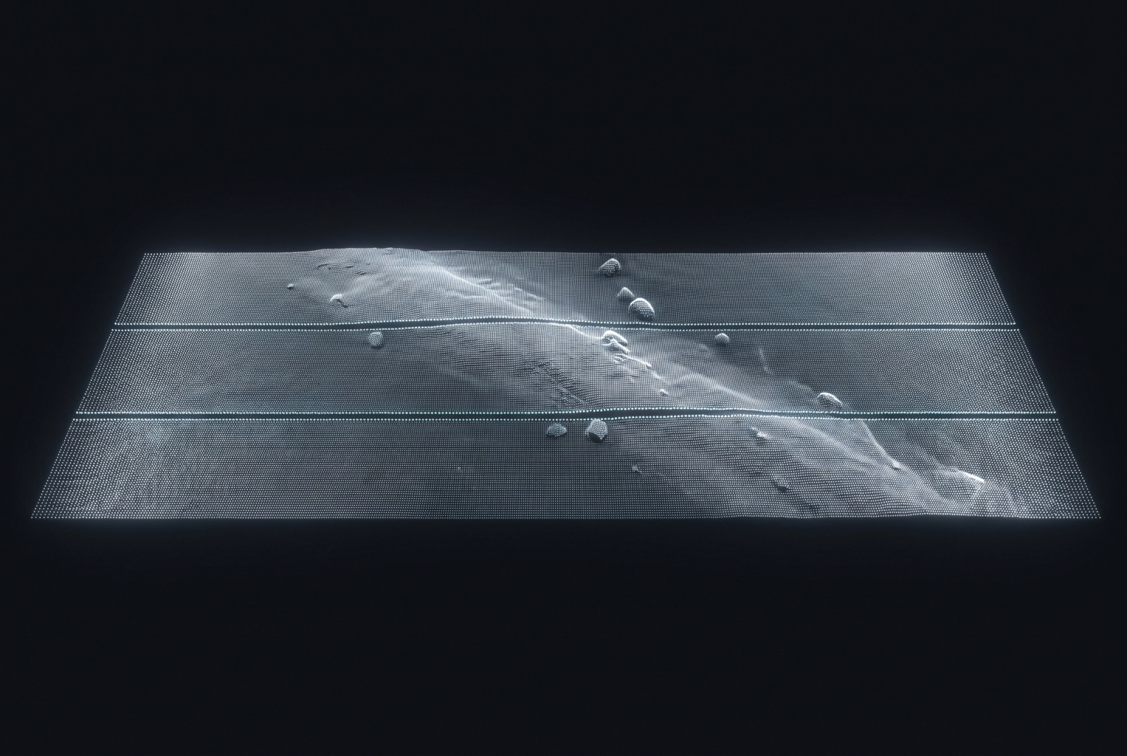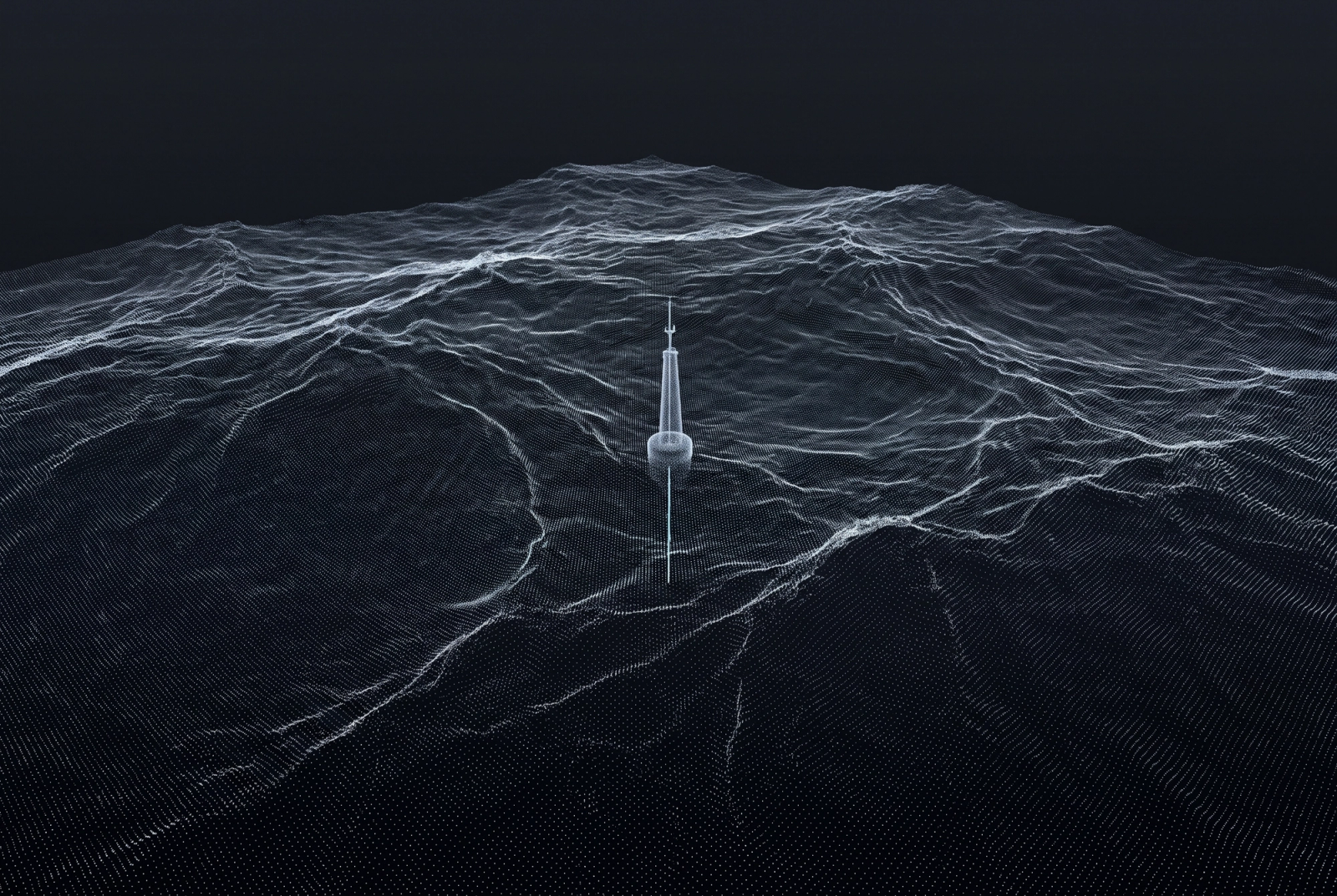
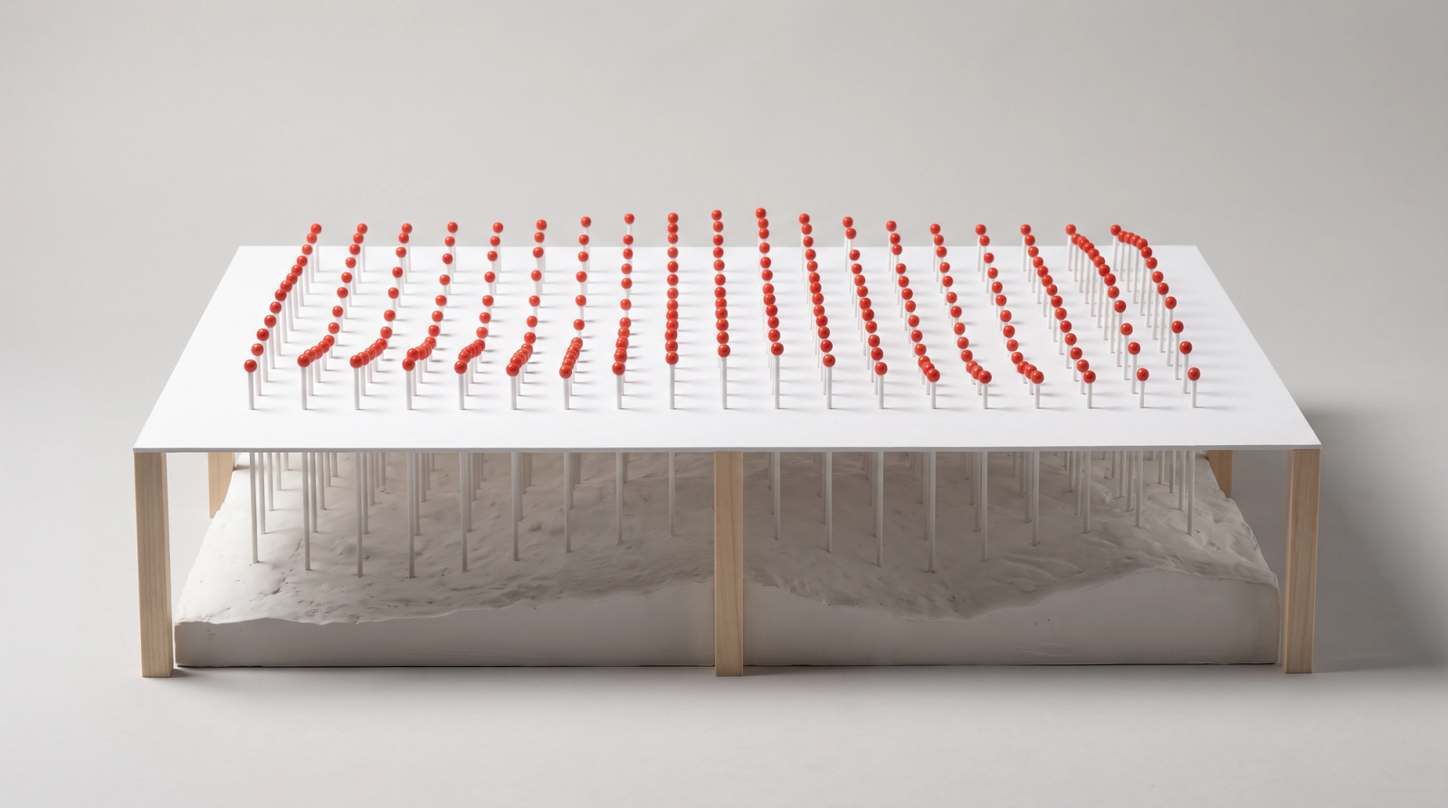
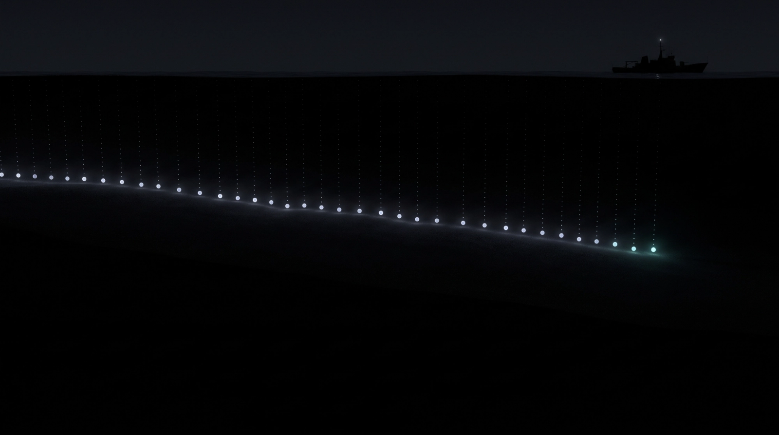
A ship lowers a weighted line and reads one number: the depth at that place, at that moment. The number is exact. It says nothing about the water a hundred metres to one side. A seafloor chart is made from many such numbers and a rule for the spaces between them, and the rule is where measurement ends and inference begins.
Methods for reading the inside of a trained network have the same shape. Each takes readings at chosen points and then has to decide how far to trust what lies between them. What follows uses bathymetry as an analogy to organise published work on probing. The analogy is flagged where it strains, and it does not claim that a network and a seabed are alike in kind.
One reading, one chart
Global seafloor grids now make the distinction explicit. The GEBCO 2024 grid is distributed with a companion grid that records, for every cell, the type of source behind its value: direct measurement (single-beam, multibeam, lidar and others) or an indirect method, including depth predicted from satellite-derived gravity[1]. A chart that labels its measured and estimated cells states what it knows and what it is filling in.
The figure below reduces this to a toy.
Hidden. Reveal it to compare with the chart.
6 soundings · average error against the hidden seabed: 5.6 m
Select a point on the chart, or focus the chart and move with the arrow keys, then press Enter to sound there. Contour lines mark every 10 metres.
How the figure works
How the figure works: the hidden seabed is a fixed surface of six smooth rises and hollows on a 48 by 28 grid. Each sounding reads the exact depth at one point. The chart fills every other point by inverse-distance weighting, each sounding weighted by one over its squared distance. The figure opens with six soundings; Start again clears them all. The error is the mean absolute difference between chart and seabed over all grid points. It illustrates inference from sparse measurement, and models neither a network nor a mind.
The figure is an illustration with fixed assumptions, stated under it. It is not a model of a neural network, and real charts use more information than the figure does, such as gravity-derived prediction[1].
Whatever the interpolation rule, two things hold. Where soundings are dense, the chart can agree closely with the seabed. Everywhere else it supplies a value that looks like the others, and a trench or ridge that falls between soundings is missing without any mark to say so. The confidence of the picture comes from the rule, not from the water.
A chart is therefore a set of predictions. The test of one is to take a sounding where it makes a claim and nothing was measured, then compare.
What a probe reads
A linear probe is a sounding. A simple classifier is trained on the activations at one layer of a network to predict a property of the input, without changing the network itself[2]. Alain and Bengio used such probes to ask how well each layer's features support classification, and reported that linear separability increased monotonically with depth in the models they tested.
The reading is exact in one sense: at this layer, on this data, this classifier recovers the property. What the reading says about the network is the chart, and the chart has the weakness described above. Hewitt and Liang made one form of that weakness measurable. A flexible probe can learn the task itself instead of reading it from the representation. Their control tasks assign random outputs to word types, so that only a probe that memorises the mapping can solve them, and selectivity is accuracy on the linguistic task minus accuracy on the control[3]. For part-of-speech tagging from the first layer of ELMo, a pretrained language model, with default settings, a one-hidden-layer perceptron probe scored 97.3 against 92.8 on the control, a selectivity of 4.5. A linear probe scored 97.2 against 71.2, a selectivity of 26.0. Task accuracy was almost the same. The control scores differ by more than twenty points, which indicates how much more capacity the perceptron probe has to score well without reading the representation.
In the analogy, a control task checks the instrument rather than the seabed. It asks how much of the reading the sounder would have produced anyway.
Decodable is not the same as used
Suppose the reading is sound. A second gap remains. Belinkov's review of the probing framework puts it directly: a probe may show a correlation between a representation and a property, but it does not show that the model's predictions involve that property[4]. A depth chart can place a ridge accurately and say nothing about where water moves across it.
Interventions are the main response. Amnesic probing removes a property from a representation, by repeatedly training linear probes and projecting out what they find, and then measures what happens to the model's behaviour. Applied to BERT, it found that conventional probing performance was not correlated with task importance[5]. Causal tracing corrupts the embeddings of the subject in a factual prompt with noise, restores one clean hidden state at one layer and position, and measures how much of the correct prediction returns. In GPT-2 XL, besides states close to the output, strong single-state effects appeared at the last token of the subject in middle layers, where feed-forward modules contributed more than attention[6]. Interchange interventions are stricter. A hypothesised high-level causal model is aligned with parts of the network, and the alignment is tested by replacing a representation with the one produced for a different input and checking that the intervened network and the intervened model give the same output[7].
These are better charts than a probe alone because they predict something that can fail. They do not remove the problem. The analogy strains here: a sounding line leaves the seabed as it was, but an intervention changes the system under study, so each causal reading carries the further question of whether the altered network still stands for the original. One inquiry on this site, what a policy holds still, asks a version of the question for a robot policy: whether the variables it defends under disturbance predict which conditions it survives better than a decoding probe does.
What a measure measures
Psychology met the same problem with tests. Cronbach and Meehl wrote that construct validation is involved whenever a test is to be interpreted as a measure of some attribute or quality that is not operationally defined, and that a construct is defined implicitly by the network of associations in which it occurs, the interlocking system of laws they called a nomological network[8]. A score alone is a sounding. Its meaning depends on how it relates to other readings, and on a theory that says what ought to move with what. Borsboom, Mellenbergh and van Heerden proposed a sparer standard: a test is valid for measuring an attribute if the attribute exists and variation in it causally produces variation in the test outcomes[9]. That is one position within validity theory and not a settled one. It can be read as the psychological counterpart of asking whether a model uses what a probe decodes.
The parallel lies in the structure of the inference. It does not show that a mind and a network resemble each other inside. Whether they do is a separate question, and this note does not answer it.



What a chart owes its reader
Two practices follow from the analogy. A claim should say which parts were measured and which were estimated, and the instrument should be checked against a case where the answer is known to be arbitrary, as control tasks do. Then the chart should be tested at a place where it makes a claim and nothing was measured, with the result that would count against it stated in advance.
The inquiry instruments for a workspace asks whether instruments that claim to measure a model's internal workspace can be trusted before they are used for anything else.
References
- GEBCO Compilation Group (2024). GEBCO 2024 Grid. General Bathymetric Chart of the Oceans (GEBCO), gridded bathymetry dataset with Type Identifier (TID) grid.
- Alain, G., Bengio, Y. (2016). Understanding intermediate layers using linear classifier probes. arXiv preprint 1610.01644.
- Hewitt, J., Liang, P. (2019). Designing and Interpreting Probes with Control Tasks. Proceedings of EMNLP-IJCNLP 2019, 2733–2743.
- Belinkov, Y. (2022). Probing Classifiers: Promises, Shortcomings, and Advances. Computational Linguistics 48(1), 207–219.
- Elazar, Y., Ravfogel, S., Jacovi, A., Goldberg, Y. (2021). Amnesic Probing: Behavioral Explanation with Amnesic Counterfactuals. Transactions of the Association for Computational Linguistics 9, 160–175.
- Meng, K., Bau, D., Andonian, A., Belinkov, Y. (2022). Locating and Editing Factual Associations in GPT. Advances in Neural Information Processing Systems 35 (NeurIPS 2022).
- Geiger, A., Lu, H., Icard, T., Potts, C. (2021). Causal Abstractions of Neural Networks. Advances in Neural Information Processing Systems 34 (NeurIPS 2021).
- Cronbach, L. J., Meehl, P. E. (1955). Construct validity in psychological tests. Psychological Bulletin 52(4), 281–302.
- Borsboom, D., Mellenbergh, G. J. and van Heerden, J. (2004). The concept of validity. Psychological Review 111(4), 1061–1071.
Cite as
Far Akin Research Labs (2026). Soundings: charting an interior you cannot see. Far Akin Research Labs. https://farakin.vercel.app/notes/soundings
@misc{farakin2026-soundings,
  title = {{Soundings: charting an interior you cannot see}},
  author = {Far Akin Research Labs},
  howpublished = {\url{https://farakin.vercel.app/notes/soundings}},
  year = {2026},
  month = oct,
  url = {https://farakin.vercel.app/notes/soundings}
}
Noticed an error or a missing source? Send a correction